In light of the recent crisis in the US, parallels are being
drawn with the infamous Lehman Brothers collapse in 2008 that shook the global
financial system. This writing aims to provide a brief exploration of the
current banking uncertainty, offering comparable information to enhance
understanding and help stakeholders mitigate future implications.
In 2007, Lehman Brothers ended its tenure as the largest real estate loan insurer in the US. Many Wall Street traders believed that the sophistication of the present century’s financial markets allowed people to take risks, and it was believed that the market, in one way or another, would have overcome this problem of high exposure. Consequently, the fall of the New York stock market starting on September 15, 2008, resulted in a loss of over $2 trillion for the global economy. The 2008/09 recession was one of the worst on record, leading to the closure of hundreds of thousands of businesses and the layoff of approximately 3.7 million people. The full cost of the current crisis is yet to be determined, but comparative aspects between 2008 and 2022 have been addressed.
Indeed, the present banking instability eerily resembles that of Lehman Brothers in 2008. In both cases, it was caused by banks taking on too much risk and then defaulting on their creditors. In the 2008 crisis, financial institutions extended a large number of high-risk mortgages, known as subprime loans, to borrowers with poor credit histories. When the housing market collapsed, many of these borrowers defaulted on their commitments, resulting in significant losses for the banking sector. Specifically for Lehman Brothers, from 2001 until September 12, 2008, the leverage ratio increased from 20 to 44 to 1. The high assumed risk caused the value of a share, which at its peak reached $85 per share, to plummet to $0.33 per share three days later. This immediate drop led to a loss of confidence in the financial system by the market and the general public, subsequently triggering a negative impact on the European and global economies.
In the current situation, banks have extended a large number of loans to businesses that are now struggling to make payments due to the COVID-19 pandemic. If these companies fail to repay their debts, it could cause financial institutions to incur significant losses and potentially lead to another financial difficulty. According to the latest Global Economic Prospects Report by the World Bank, the damages caused by the COVID-19 pandemic, the Russian invasion of Ukraine, the lockdowns in China, supply chain disruptions, and the risk of stagflation have exacerbated the global economic slowdown, entering a prolonged period of low growth and high inflation.
Similarities and differences between the crises: While the current banking crisis shares similarities with the Lehman Brothers crisis of 2008, it is important to recognize key differences that distinguish these two events. Both crises were generally caused by a combination of endogenous factors, including economic, political, and social aspects. However, the 2022 crisis had a health-related issue, an unforeseen factor that significantly impacted civil society, leading to calls for reform and change. Understanding both the similarities and differences can provide valuable insights into the nature and potential outcomes of the current crisis. Let’s explore these aspects in more detail:
Coincidences:
a. Systemic risk: Both crises have exposed systemic risks within the global financial system. The collapse of Lehman Brothers in 2008 and the current crisis have demonstrated how vulnerabilities in the banking sector can have far-reaching implications, affecting not only financial institutions but also the overall economy.
b. Excessive risk-taking: In both cases, excessive risk-taking by financial institutions played a significant role. The pursuit of higher profits and returns led to the adoption of risky lending practices and the creation of complex financial products. These practices amplified the potential for financial instability and contagion.
c. Economic impacts: The consequences of both crises have had severe economic impacts. The 2008 crisis resulted in a global recession, characterized by a sharp decline in economic activity, job losses, and a reduction in consumer and investor confidence. Similarly, the current crisis has the potential to disrupt economic growth, increase unemployment and inflation rates, and negatively affect market confidence.
Differences:
a. Triggers: The triggers of the crises differ significantly. The Lehman Brothers crisis was largely driven by the bursting of the U.S. housing bubble and the subsequent collapse of the high-risk mortgage market. In contrast, the current crisis may have multiple triggers, such as geopolitical tensions, rising levels of debt, and economic imbalances exacerbated by the COVID-19 pandemic.
b. Regulatory reforms: Following the Lehman Brothers crisis, regulatory reforms were implemented to strengthen the banking sector and improve financial stability. These reforms aimed to address the vulnerabilities and deficiencies exposed by the crisis. However, the effectiveness of these measures and their impact on the current crisis may vary depending on specific regulatory frameworks in place.
c. Global economic context: The global economic context surrounding the two crises is different. The Lehman Brothers crisis occurred during a period of overall economic growth, whereas the current crisis unfolds amidst the aftermath of a global pandemic. The unique challenges and uncertainties posed by the pandemic add a layer of complexity to the current crisis.
In conclusion, while the current banking crisis shares similarities with the Lehman Brothers crisis of 2008, it is essential to recognize the differences in triggers, regulatory response, and the global economic context. Understanding these similarities and differences can provide valuable insights into the possible implications and outcomes of the current crisis. One significant difference identified is the behavior of inflation and its antecedents as a catalyst for the current crisis. Therefore, the fundamentals that did not coincide between the crises will be evaluated, considering their importance, and discussed below.
Quantitative easing (QE) is a monetary policy action in which a central bank purchases predetermined amounts of government bonds or other financial assets to stimulate economic activity. QE is a novel form of monetary policy that came into widespread use after the 2007–2008 financial crisis. It is used to mitigate an economic recession when inflation is very low or negative, rendering standard monetary policy ineffective. As of May 2023, the money supply in the US is $20.82 trillion. This is the total amount of money available in the US economy. Figure 1 illustrates the steep growth of the money supply, particularly over the past three years.

To illustrate the functioning of quantitative easing, consider some of the evidence used in the last decade:
- Increasing the money supply: When the central bank purchases assets, it creates new money. This increases the amount of money available in the economy, which can lead to lower interest rates and, consequently, an increased need for borrowing.
- Reducing interest rates: When the central bank buys assets, it increases the demand for them. This drives up asset prices, which lowers their yields. Lower yields make it cheaper for businesses and consumers to borrow money, which can lead to increased investment and spending.
- Providing liquidity to the financial system: When the central bank purchases assets, it injects cash into the financial system. This can help stabilize the financial system and prevent a liquidity crisis.
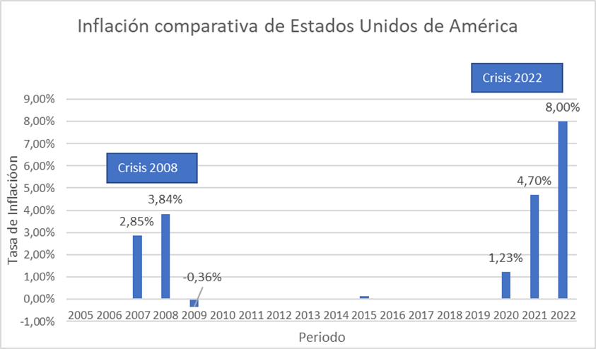
Inflation: One of the key differences between the crises relates to changes in the consumer price index (CPI). The comparative inflation rate (7) during the peak levels of the crises shows a notable differential behavior. While in 2008 it reached 3.84%, with a subsequent deflationary decrease of -0.36% the following year, by 2022, this index reached 8%, as shown in the Figure below.

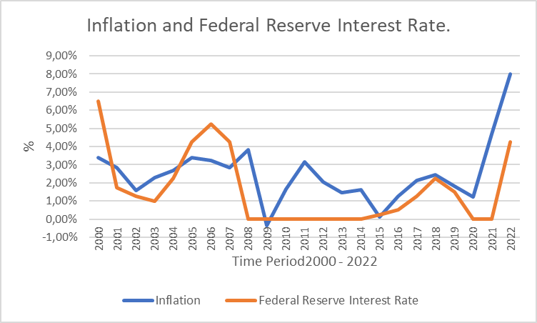
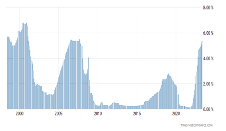
In theory, inflation precedes the behavior of interest rates, and interest rates react directly to inflationary patterns. In monetary policy, the adjustment of interest rates serves two purposes. First, it aims to stimulate economic growth during recessions by lowering rates to 0% when desired inflation rates are under control within a moderate range of around 2%. This can be observed in Figure 3 during the period from late 2008 to 2014, following the subprime crisis. This policy allows economic entities to borrow at low rates, encouraging the supply of goods and services to enter the market. Second, it aims to control inflationary growth by raising interest rates, as is happening at present.
Based on these considerations, it is likely that interest rates will remain elevated for some time. This does not imply a further increase in rates, but rather serves as a tool to curb inflation, maintaining high rates that can dampen inflationary growth and eventually break its upward trend. As shown in Figure 3, inflation has been significantly higher than the interest rates set by the Fed since 2020, supporting the hypothesis put forward.

Indeed, the relationship between inflation and interest rates is complex and dynamic, particularly in the context of the current crisis. Here are some arguments and perspectives on this topic:
Inflationary Pressures: The current crisis has introduced unique inflationary pressures. On one hand, disruptions in supply chains, reduced production, and rising production costs can create upward pressure on prices. On the other hand, weakened consumer demand and high unemployment rates can exert downward pressure on prices. The scope and duration of these inflationary pressures remain uncertain.
Central Bank Response: Central banks, including the Federal Reserve, closely monitor inflation dynamics when formulating monetary policy. In response to increasing inflationary pressures, central banks may consider raising interest rates to curb inflation and maintain price stability. Conversely, in a low-inflation environment, central banks may opt to keep interest rates low to stimulate economic activity and foster inflation.
Economic Recovery: The relationship between inflation and interest rates in the current crisis is also intertwined to promote economic recovery. Central banks may prioritize supporting economic growth and employment over immediate concerns about inflation. Therefore, they may maintain accommodative monetary policies, such as low-interest rates, to encourage borrowing, investment, and consumption.
Impact on Borrowers and Savers: The relationship between inflation and interest rates has implications for borrowers and savers. In a low-interest-rate environment, borrowing costs can be favorable for individuals and businesses, promoting investment and economic growth. However, savers may experience lower returns on their savings, which could affect their ability to accumulate wealth over time.
Inflation Expectations: Inflation expectations play a crucial role in the relationship between inflation and interest rates. If individuals and businesses anticipate higher inflation in the future, they may demand higher interest rates to compensate for the erosion of purchasing power. Central banks closely monitor and manage these expectations through communication and policy actions.
Unconventional Monetary Policies: In addition to conventional interest rate adjustments, central banks can employ unconventional monetary policies, such as quantitative easing, to address inflation and stimulate economic activity. These policies involve the purchase of government bonds or other financial assets to increase the money supply and influence interest rates.
Interest Rates and Public Debt
Another aspect to highlight is the behavior of U.S. Treasury bonds, considered global reserve assets. Due to high widespread inflation, the monetary policy establishes at least two mechanisms for inflation control. The first involves restricting consumer credit in the market, a measure that is rarely implemented to avoid disruption of economic activities. However, this restriction leads to the issuance of new bonds, which often compete with market rates demanded by investors, adjusted to prevailing inflation. This mechanism has contributed to U.S. national debt reaching $31.5 trillion as of February 15, 2023. This is the total amount of money that the U.S. government owes to its creditors, including individuals, businesses, and foreign states. These funds have been borrowed to finance government expenses since the early 19th century. These obligations have steadily grown over time, reaching record levels in recent years. State debt is financed through the sale of bonds. Bonds are a type of loan that the government makes to investors. Investors buy bonds because they are considered a safe investment, based on a long history of timely payment of their liabilities.
From the aforementioned, it can be inferred that U.S. national debt is one of the main concerns for economists and policymakers. It is so large that it is now considered a threat to the U.S. economy. Government interest payments on the debt are now the third largest item in the federal budget. If it continues to grow, it could eventually lead to a financial crisis.
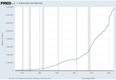
So, the question arises: What should the Federal Reserve (Fed) and the U.S. Treasury do to address this systemic situation? There are at least a couple of actions the U.S. government could take to reduce the national debt. One option would be to increase taxes. Another option, and the more suitable one, would be to cut spending. However, both options are politically unpopular. U.S. national debt will likely continue to grow in the coming years. Figure 4 below presents historical data that supports this statement.


Graph 4 shows that U.S. debt has steadily increased over the past 40 years. In 1982, the debt was $1.2 trillion. By 2022, the debt had risen to $31.5 trillion, representing an increase of over 2500%.
The second measure is the increase in interest rates, which has historically been a reliable tool to deflate the economy. However, this mechanism has its modus operandi, which simultaneously affects bond yields. Issuing new long-term bonds with higher yields attracts investors who may convert their short and medium-term savings or investments into immediate cash to reinvest in current bonds. Implicitly, this mechanism is beneficial from an investor’s perspective, but for banks that have maintained significant gaps between their liabilities and assets for a long time, it has caused liquidity imbalances. They may have to resort to interbank loans or sell their longer-term positions at very low rates. As can be seen, when those old bond investments are cashed in, there is an automatic loss in the value of those bonds due to the discount rate at which the market would be willing to buy them.
If this scenario is evident for a simple investor, now let’s think about what happens with large investors or even countries that have invested their reserves in low-yield American bonds. It is clear to infer that there is a contingency in national balances when it becomes necessary to liquidate assets to meet liquidity needs for banks, investors, and states in general.
As a corollary to the above, in a recent article citing the Federal Deposit Insurance Corp. on the total number of bank failures, the author records 513 banks that have closed their operations from 2009 to 2023, of which three banks, Silicon Valley Bank, Signature Bank New York, and First Republic Bank, closed their operations in the last quarter.
Some reflections
But the question is, what should states, represented by their leaders, do to avoid repeating what has already been mentioned? Several measures come to mind that the government can take to prevent another financial crisis. First, it can regulate banks more closely to ensure they don’t take on excessive risks. Second, it can provide financial assistance to banks that are at risk of failing. Third, it can work to stabilize the financial markets. The U.S. government has already taken some steps to prevent another financial crisis. In 2010, it passed the Dodd-Frank Wall Street Reform and Consumer Protection Act, which was specifically designed to make the financial system more stable. Additionally, it is worth noting that during the Donald Trump administration (2017–2021), some laws were deregulated, such as the Law of Economic Growth, Regulatory Relief, and Consumer Protection of 2018, specifically aimed at favoring the financial sector, for example, by (i) establishing lower capital requirements and leverage ratios, (ii) exempting deposit requirements for residential mortgage loans held by a depository institution or credit union under certain conditions, and (iii) exempting lenders with assets below $10 billion from Volcker Rule requirements.
Referring to the second question, for example, states have also provided financial assistance to banks during the COVID-19 pandemic. However, more needs to be done to prevent another financial crisis. The government should continue to regulate banks more closely and work to stabilize the financial markets.
As mentioned, the current banking crisis is a serious threat to the global economy. Measures must be taken to prevent another financial crisis. By regulating banks more closely, providing financial assistance to those at risk of failing, and working to stabilize the financial markets, governments can help prevent another financial crisis and protect the global economy. In this sense, not only private investors or companies are facing this contingency, even countries holding American debt or those countries whose sovereign assets have been valued at low average rates in the last 10 years. Therefore, it is presumed that the global financial system would be at serious risk.
Conclusion
COVID-19 was the main cause of the current crisis.
Undoubtedly, this unforeseen exogenous factor was the trigger for an underlying reality that caused such an imbalance that it revealed an unprogrammed increase in quantitative easing, resulting in demand-driven inflation and a simultaneous decrease in global supply.
Improving provisions
I once had a conversation with a close friend, and when discussing this topic, he said that making provisions for such contingencies would mean disclosing a financial position that could be detrimental to the company. Indeed, it is detrimental, but it is even worse to have to realize those assets at the current moment, considering that American bonds will remain at attractively high rates until at least 2024. Regulators should expect higher levels of provisions during times of high systematic risk.
Prevention and control of inflation
In conclusion, the relationship between inflation and interest rates in the current crisis is influenced by several factors, including inflationary pressures, central bank responses, economic recovery goals, dynamics of borrowers and savers, inflation expectations, and unconventional monetary policies. Central banks carefully analyze these factors to make informed decisions on interest rates and monetary policy, aiming to strike a balance between price stability and supporting economic growth.
Investing in bonds is not necessarily safe.
The question is how to hold onto bonds with low rates during an impending recession. Not only will you face illiquidity, but you will also inexorably deplete capital until the economy returns to a growth trajectory. This is a complex and crucial issue that would warrant a more detailed discussion.
References
1. Merle R. A guide to the financial crisis — 10 years later. Washington Post [Internet]. 10 de septiembre de 2018 [citado 14 de mayo de 2023]; Disponible en: https://www.washingtonpost.com/business/economy/a-guide-to-the-financial-crisis--10-years-later/2018/09/10/114b76ba-af10-11e8-a20b-5f4f84429666_story.html
2. Bondarenko. 5 of the World’s Most Devastating Financial Crises | Britannica [Internet]. sf [citado 14 de mayo de 2023]. Disponible en: https://www.britannica.com/list/5-of-the-worlds-most-devastating-financial-crises
3. Bachelor-Hunt. Cost of living crisis: 2022 «could be worse than the financial crisis» [Internet]. Yahoo News. 2022 [citado 14 de mayo de 2023]. Disponible en: https://uk.news.yahoo.com/2022-could-be-worse-than-financial-crisis-113251144.html
4. Daniel W. 3 key differences between the economy today and the pre-Great Recession era [Internet]. Fortune. 2022 [citado 14 de mayo de 2023]. Disponible en: https://fortune.com/2022/03/26/great-recession-key-differences-us-economy-inflation/
5. Banco Mundial. Perspectivas económicas mundiales junio 2022 [Internet]. World Bank. 2022 [citado 30 de octubre de 2022]. Disponible en: https://www.bancomundial.org/es/news/press-release/2022/06/07/stagflation-risk-rises-amid-sharp-slowdown-in-growth-energy-markets
6. U.S. Department of the Treasury. Fiscal Service. Federal Debt: Total Public Debt [Internet]. FRED, Federal Reserve Bank of St. Louis. FRED, Federal Reserve Bank of St. Louis; 1966 [citado 16 de mayo de 2023]. Disponible en: https://fred.stlouisfed.org/series/GFDEBTN
7. DatosMundial.com. Tasas inflacionarias en los Estados Unidos de América [Internet]. DatosMundial.com. 2023 [citado 15 de mayo de 2023]. Disponible en: https://www.datosmundial.com/america/usa/inflacion.php
8. Trading Economics. Estados Unidos — Tasa de interés interbancaria | 1986–2023 Datos [Internet]. 2023 [citado 15 de mayo de 2023]. Disponible en: https://es.tradingeconomics.com/united-states/interbank-rate
9. Datosmacro.com. Tipos de la Reserva Federal de USA 2023 | [Internet]. 2023 [citado 15 de mayo de 2023]. Disponible en: https://datosmacro.expansion.com/tipo-interes/usa
10. Goldberg M. List Of Failed Banks: 2009–2023 [Internet]. Bankrate. 2023 [citado 16 de mayo de 2023]. Disponible en: https://www.bankrate.com/banking/list-of-failed-banks/

